The Fusion of Deep Learning and Combinatorics

(authored by Marin Vlastelica)

Breakthrough: how can we seamlessly incorporate combinatorial solvers in deep neural networks. A summary of our ICLR 2020 spotlight paper.

The current landscape of machine learning research suggests that modern methods based on deep learning are at odds with good old-fashioned AI methods. Deep learning has proven to be a very powerful tool for feature extraction in various domains, such as computer vision, reinforcement learning, optimal control, natural language processing and so forth. Unfortunately, deep learning has an Achilles heel, the fact that it cannot deal with problems that require combinatorial generalization. An example is learning to predict quickest routes in Google Maps based on map input as an image, an instance of the Shortest Path Problem. A plethora of such problems exists like (Min,Max)-Cut, Min-Cost Perfect Matching, Travelling Salesman, Graph Matching and more.

But if such combinatorial problems are to be solved in isolation, we have an amazing toolbox of solvers available, ranging from efficient C implementations of algorithms to more general MIP (Mixed Integer Programming) solvers such as Gurobi. The problems that the solvers face are in the representation of the input space since the solvers require well-defined, structured input.

Although combinatorial problems have been a subject in the machine learning research community, the attention towards solving such problems has been lacking. This doesn’t mean that the problem of combinatorial generalization has not been identified as a crucial challenge on the path to intelligent systems. Ideally, one would be able to combine the rich feature extraction available through powerful function approximators, such as neural networks, with the efficient combinatorial solvers in an end-to-end manner without any compromises. This is exactly what we were able to achieve in our recent paper [1] for which we have received top review scores and are giving a spotlight talk at ICLR 2020.

For the following sections, it’s worth keeping in mind that we are not trying to improve the solvers themselves, but rather enable usage of existing solvers in synergy with function approximation.

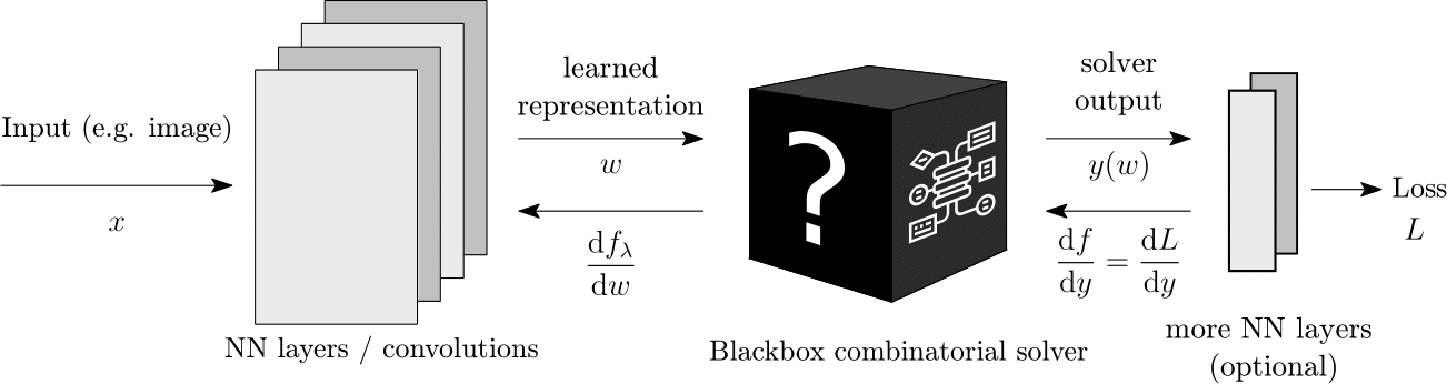We imagine a blackbox solver as an architectural module for deep learning that we can simply plug in.

Gradients of Blackbox Solvers

The way we think about combinatorial solvers is in terms of a mapping between a continuous input (e.g. weights of graph edges) to a discrete output (e.g. shortest path, selected graph edges), defined as

The solver minimizes some kind of cost function c(ω,y), for instance, the length of the path. More concretely, the solvers solves the following optimization problem:

Now, imagine that ω is the output of a neural network, i.e. is some kind of representation that we learn. Intuitively, what does this ω mean? ω serves the purpose of defining the instance of the combinatorial problem. As an example, ω can be a certain vector that defines the edge weights of a graph. In this case, the solver can solve the Shortest Path Problem or the Travelling Salesman, or whichever problem we want to be solved for the specified edge costs. The thing that we want to achieve is the correct problem specification through ω.

Naturally, we want to optimize our representation such that it minimizes the loss which is a function of the output of the solver L(y). The problem that we are facing right away is the fact that the loss function is piecewise-constant, meaning the gradient of this function with respect to the representation ω is 0 almost everywhere and undefined on the jumps of the loss function. Put more bluntly, the gradient as-is is useless for minimizing the loss function.

Till now there have been approaches relying on solver relaxations, where sacrifices had to be made with regards to its optimality. In comparison, we have developed a method without compromises to the optimality of the solver. We achieve this by defining a piecewise affine interpolation of the original objective function where the interpolation itself is controlled by a hyperparameter λ, as shown in the following figure:

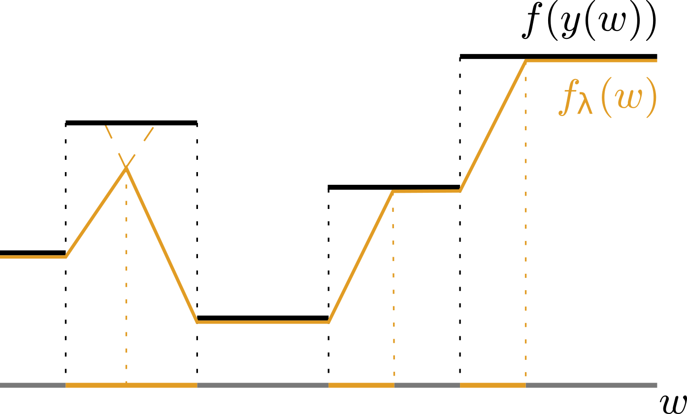
As we can see, f (black) is piecewise constant. Our interpolation (orange) connects the plateaus in a reasonable fashion. For instance, notice that the minimum is not changed.

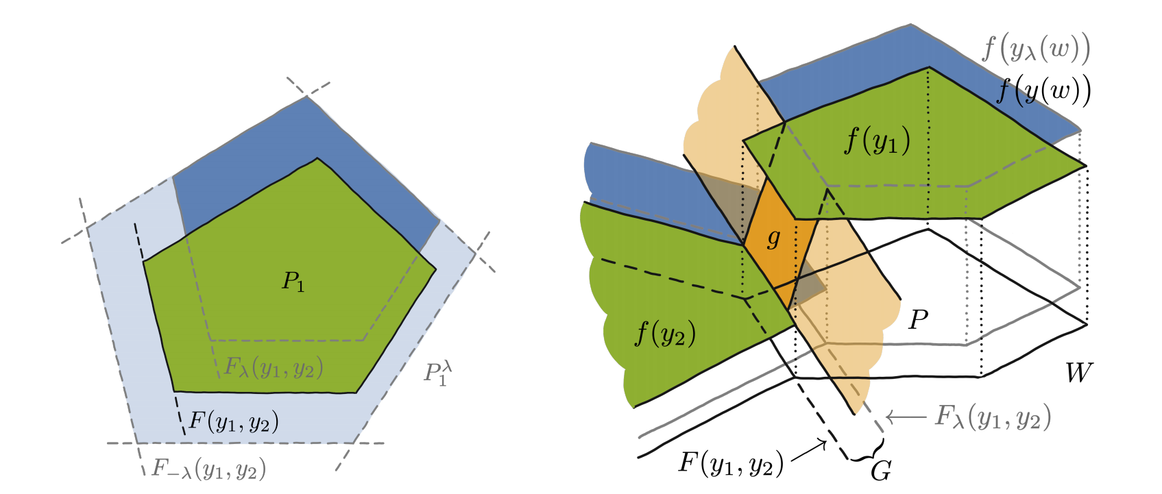
The domain of f is, of course, multi-dimensional. As such, we can observe the set of inputs ω for which f obtains the same value as a polytope. Naturally, there are many such polytopes in the domain of f. What the hyperparameter λ effectively does is that it shifts the polytopes through the perturbation of the input of the solver, ω. The g interpolators that define the piecewise-affine objective connect the shifted boundary of the polytope to the original boundary. Such a situation is depicted in the lower figure, where the boundary of the polytope that obtains the value f(y2) is shifted to obtain the value of f(y1). This also intuitively explains why higher values of λ are preferable. The shifts have to be big enough to obtain the interpolator g which is going to provide us with an informative gradient. Proofs can be found in [1].

First, let us define a solution to the perturbed optimization problem, where the perturbation is controlled by the hyperparameter λ:

If we assume that the cost function c(ω,y) is a dot product between y and ω, we can define the interpolated objective like the following:

Note that the linearity of the cost function is not as restrictive as it might seem at first glance. All problems involving edge selection, where the cost is the sum of the edge weights fall into this category. The Shortest Path Problem (SPP) and Travelling Salesman Problem (TSP) are examples that belong to this category of problems.

The Algorithm

With our method, we were able to remove the rift between classical combinatorial solvers and deep learning with a simple modification to the backward pass to calculate the gradient.

The computational overhead of calculating the gradient of the interpolation depends on the solver, the additional overhead is calling the solver once on the forward pass and once on the backward pass.

Experiments

We have developed synthetic tasks that contain a certain level of combinatorial complexity to validate the method. In the following tasks, we have shown that our method is essential for combinatorial generalization since naive supervised learning approaches fail at generalizing to unseen data. Again, the goal is to learn the correct specification of the combinatorial problem.

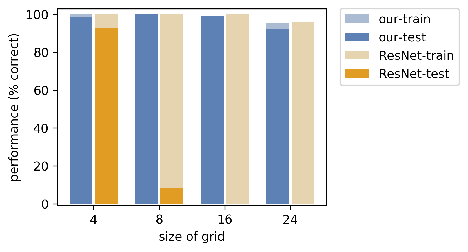
For the Warcraft Shortest Path problem, the training set consists of Warcraft II maps and corresponding shortest paths on the maps as targets. The test set consists of unseen Warcraft II maps. The maps themselves encode a k × k grid. The maps are inputs to a convolutional neural network which outputs the vertex costs for the map that are fed to the solver. Finally, the solver, which is effectively Dijkstra’s shortest path algorithm, outputs the shortest path on the map in the form of an indicator matrix.

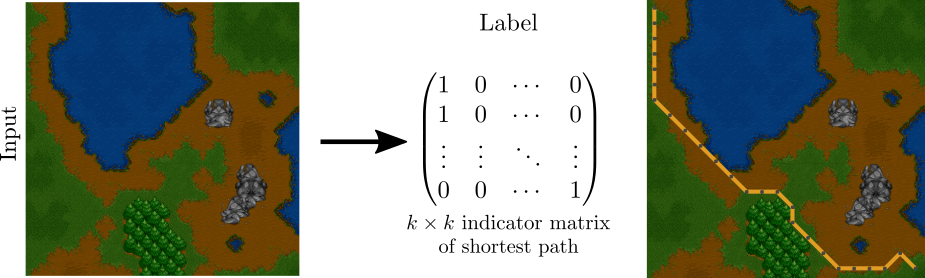
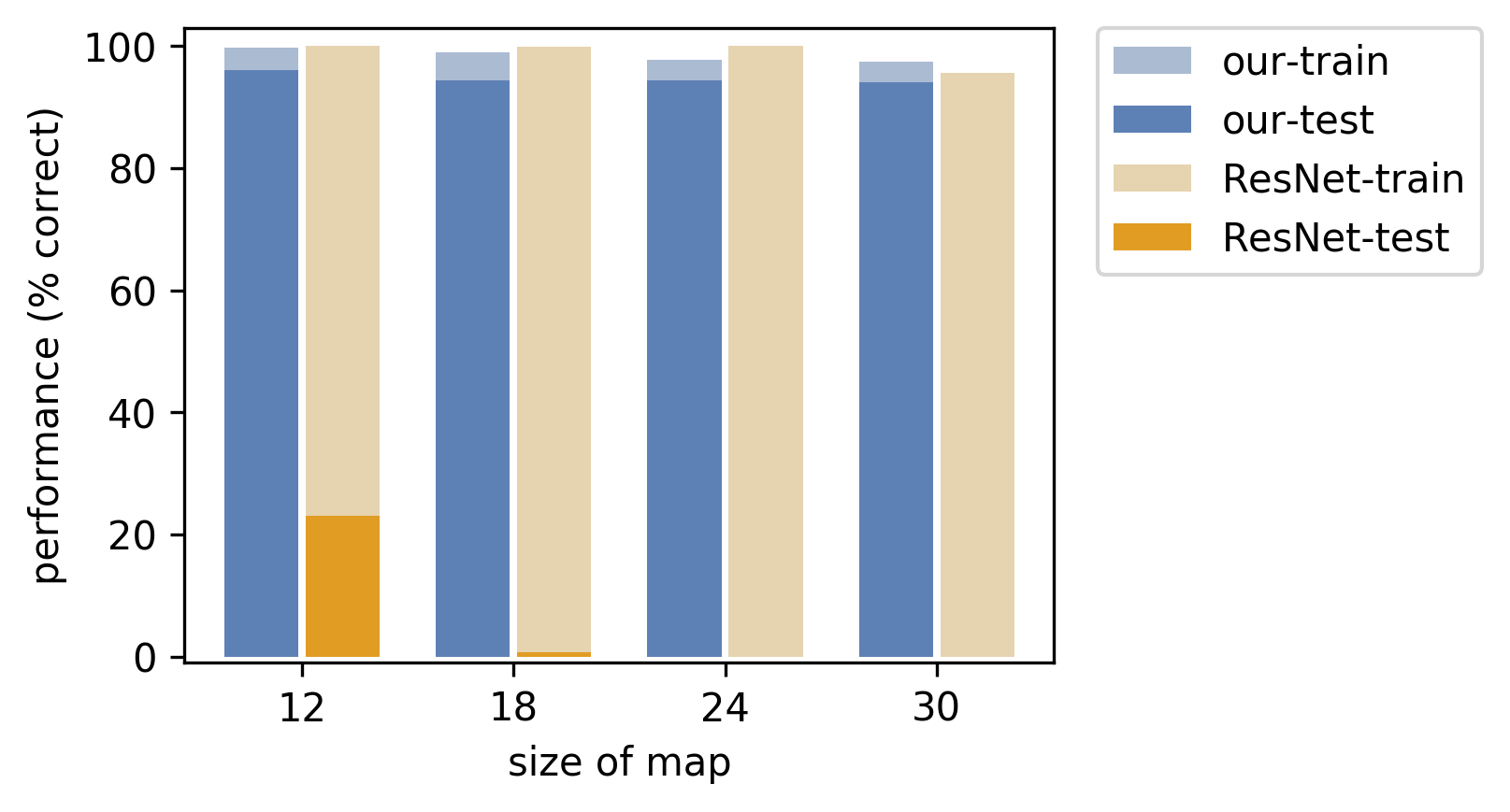
Naturally, at the beginning of training, the network doesn’t know how to assign correct costs to the tiles of the map, but with our method, we’re able to learn the correct tile costs and therefore the correct shortest path. The histogram plot shows how our method is able to generalize **significantly **better than traditional supervised training of the ResNet.

In the MNIST Min-Cost Perfect Matching problem, the goal is to output a min-cost perfect matching of a grid of MNIST digits. Concretely, in the min-cost perfect matching problem, we are supposed to select edges such that all vertices are contained in the selection exactly once and the sum of the edge costs is minimal. Each cell in the grid contains an MNIST digit that is a node in the graph having vertical and horizontal neighbors. The edge costs are determined by reading the two-digit number vertically downwards or horizontally to the right.

For this problem, a convolutional neural net (CNN) receives as input the image of the MNIST grid and outputs a grid of vertex costs that are transformed into edge costs. The edge formulation is then given to the Blossom V perfect matching solver.

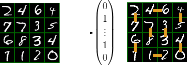
The solver outputs an indicator vector of edges selected in the matching. The cost of the matching on the right is 348 (46 + 12 horizontally and 27 + 45 + 40 + 67 + 78 + 33 vertically).

Again, in the performance plot, we notice a clear advantage of embedding an actual perfect matching solver in the neural network.

We also looked at a formulation of the **Travelling Salesman Problem **where the network is supposed to output optimal TSP tours of country capitals. For this problem, it is important to learn the correct capital positions in the latent representation. Our dataset consisted of country flags (i.e. the raw representation) and optimal tours of the respective capitals. A training example consists of **k **countries. In this case, a convolutional neural network is shown a concatenation of the country flags and is supposed to output the optimal tour.

(5)

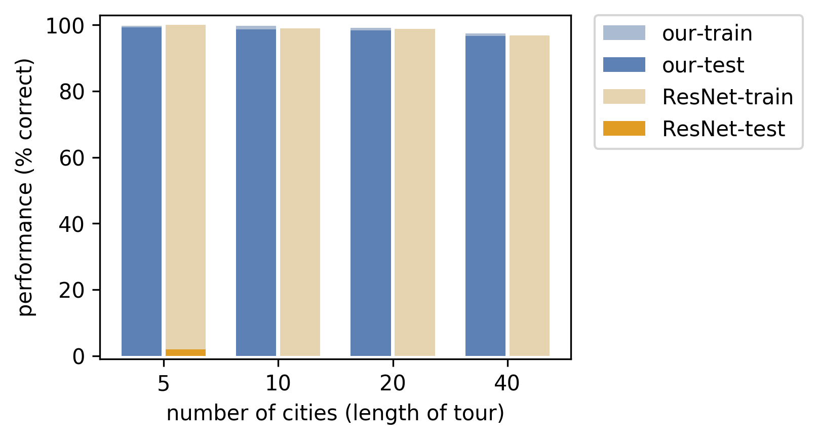
In the following animation, we can see the learned locations of the countries’ capitals on the globe during training time. In the beginning, the locations are scattered randomly, but after training the neural network not only learns to output the correct TSP tours, but also the correct representation, i.e. the correct 3D coordinates of the individual capitals. Notably, this follows from merely using the Hamming distance loss for supervision and a Mixed Integer Program in Gurobi on the outputs of the network.

Conclusion

We have shown that we can, in fact, propagate gradients through blackbox combinatorial solvers under certain assumptions about the cost function of the solver. This enables us to achieve combinatorial generalization of which standard neural network architectures are incapable based on traditional supervision.

We are in the process of showing that this method has a wide range of applications in tackling real-world problems that require combinatorial reasoning. We have already demonstrated one such application addressing rank-based metric optimization [2]. The question remains however how far away (in theory and in practice) can we go from the linearity assumption of the solver’s cost. Another question for future work is if we can learn the underlying constraints of the combinatorial problem in a MIP formulation as an example. The application spectrum of such approaches is broad and we welcome anyone that is willing to collaborate on extending this work to its full potential.

References

[1] Vlastelica, Marin, et al. “Differentiation of Blackbox Combinatorial Solvers” ICLR 2020.

[2] Rolínek, Michal, et al. “Optimizing Rank-based Metrics with Blackbox Differentiation” CVPR 2020 (oral).

Acknowledgment

This is joint work from the Autonomous Learning Group of the Max Planck Institute for Intelligent Systems and Universita degli Studi di Firenze, Italy.